What problem does this solve?
Many problems break into smaller versions of themselves, and the small versions repeat. Computing them independently wastes exponential effort; computing each once and reusing the answer turns an intractable recursion into a table you can fill in polynomial (or pseudo-polynomial) time.
Dynamic programming (DP) is the discipline of doing that deliberately. It solves combinatorial problems like knapsack, shortest paths, sequence alignment, and scheduling, and, in its Bellman-equation form, it is the mathematical foundation for decisions made over time under uncertainty: inventory replenishment, asset management, routing with stochastic travel times.
When should you use it?
Two properties must hold.
- Optimal substructure. An optimal solution contains optimal solutions to its subproblems. The best path from A to C through B uses the best path from A to B.
- Overlapping subproblems. The same subproblems recur. If they did not, plain recursion (divide and conquer) would do.
A practical test: can you describe the problem with a small state that summarizes everything the future depends on? If the state is small enough to enumerate, DP is usually the right tool. If it is too large, approximate dynamic programming or reinforcement learning take over.
Mathematical formulation
The general form is the Bellman equation. With state , decision from feasible set , immediate contribution , and next state ,
Under uncertainty, with random information arriving after the decision and a discount factor ,
The solution is not a single answer but a policy: a rule that maps any state to the best decision.
For the 0/1 knapsack problem, with items of weight and value and capacity , the state is (items considered, capacity left) and
Intuition
There are two ways to exploit overlapping subproblems.
- Top-down with memoization. Write the natural recursion, and cache each result the first time you compute it. Only the subproblems you actually reach get solved.
- Bottom-up tabulation. Fill a table in an order where every entry’s dependencies are already computed. No recursion, predictable memory, and easy to reconstruct the solution.
Fibonacci is the smallest example. The naive recursion recomputes , , and so on exponentially many times; with a cache, each value is computed once. The memoization diagram on the Optimization page shows the recursion tree collapsing.
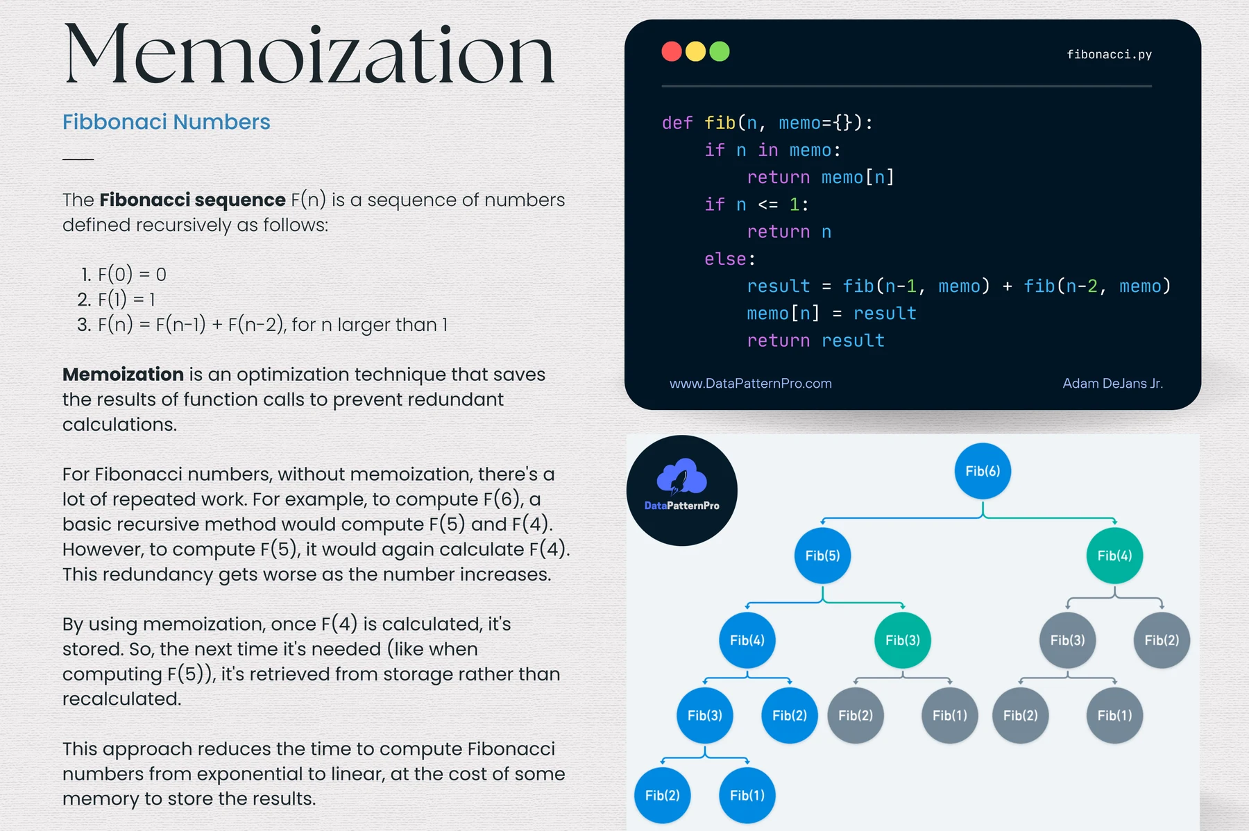
Memoization turns the exponential Fibonacci recursion into a linear one. From the original Data Pattern Pro optimization references.
The deeper intuition is in the Bellman equation: you never need to remember how you got to a state, only how good it is to be there. That is what lets a sequential decision collapse into a table of state values.
Worked example
Pack a bag with capacity 10:
| Item | Weight | Value | Value per unit weight |
|---|---|---|---|
| A | 5 | 60 | 12.0 |
| B | 4 | 40 | 10.0 |
| C | 6 | 66 | 11.0 |
| D | 3 | 27 | 9.0 |
Greedy by value density takes A (12.0), cannot fit C next (5 + 6 > 10), takes B, and stops at weight 9 with value 100.
DP fills the table row by row:
| Items considered \ capacity | 0 | 3 | 4 | 5 | 6 | 7 | 8 | 9 | 10 |
|---|---|---|---|---|---|---|---|---|---|
| none | 0 | 0 | 0 | 0 | 0 | 0 | 0 | 0 | 0 |
| A | 0 | 0 | 0 | 60 | 60 | 60 | 60 | 60 | 60 |
| A, B | 0 | 0 | 40 | 60 | 60 | 60 | 60 | 100 | 100 |
| A, B, C | 0 | 0 | 40 | 60 | 66 | 66 | 66 | 100 | 106 |
| A, B, C, D | 0 | 27 | 40 | 60 | 66 | 67 | 87 | 100 | 106 |
The optimum is 106: items B and C, using the full capacity. Tracing back from the bottom-right cell recovers the choice. Greedy was 6% worse, and on larger instances the gap can be much bigger. The LP relaxation (allowing fractions of items) gives an upper bound of 115, which is how a branch and bound solver would prune.
Python implementation
from functools import lru_cache

def knapsack(weights, values, capacity):
    """Bottom-up 0/1 knapsack. Returns (best value, chosen item indices)."""
    n = len(weights)
    V = [[0] * (capacity + 1) for _ in range(n + 1)]
    for i in range(1, n + 1):
        w, v = weights[i - 1], values[i - 1]
        for c in range(capacity + 1):
            V[i][c] = V[i - 1][c]
            if w <= c:
                V[i][c] = max(V[i][c], v + V[i - 1][c - w])
    chosen, c = [], capacity                     # trace back the decisions
    for i in range(n, 0, -1):
        if V[i][c] != V[i - 1][c]:
            chosen.append(i - 1)
            c -= weights[i - 1]
    return V[n][capacity], sorted(chosen)

print(knapsack([5, 4, 6, 3], [60, 40, 66, 27], 10))   # (106, [1, 2]) -> B and C

@lru_cache(maxsize=None)
def fib(n):
    """Top-down with memoization: each fib(k) is computed once."""
    return n if n < 2 else fib(n - 1) + fib(n - 2)

print(fib(90))   # instant; the naive recursion would take centuries
Interactive demonstration
An interactive DP explorer is planned for the playground. Until then, the Critical Ratio Explorer shows the single-period case that multi-period inventory DPs build on.
Computational complexity and trade-offs
- Cost = number of states × work per state. Knapsack has states with work each, so time. That is pseudo-polynomial: polynomial in the numeric value of , exponential in its number of digits.
- Memory can often be cut from to by keeping one row, at the cost of a harder trace-back.
- Top-down vs bottom-up. Memoization solves only reachable states and is easier to write; tabulation avoids recursion limits and has better cache behavior.
- The curse of dimensionality. With several state variables, the table grows exponentially. Inventory across 10 warehouses, each with 100 possible levels, has states. That is where approximate dynamic programming, value function approximation, and policy search come in.
Common mistakes
- A state that does not summarize the past. If the future depends on something the state omits, the recursion is wrong, not just slow.
- Using DP where greedy is provably optimal, such as fractional knapsack or activity selection. DP still works but is unnecessary.
- Using greedy where it is not, as in the example above.
- Forgetting to reconstruct the decisions. The value table alone does not tell you what to do; store choices or trace back.
- Ignoring pseudo-polynomial blow-up. Capacities in the millions make a “fast” DP slow; scale or round the weights, or switch to branch and bound.
- Treating a deterministic plan as a policy. Under uncertainty, the DP’s output is a rule for every state, which is what makes it robust to surprises. See Rethinking MILP as a Policy.
Related patterns
Knapsack problems
Choose the most valuable subset that fits a capacity; the prototype of combinatorial selection.
Markov decision processes
States, actions, transition probabilities, and rewards: the language of sequential decisions.
Approximate dynamic programming
When the state space is too large to enumerate, approximate the value function.
Greedy algorithms
Take the locally best step; know exactly when that is globally optimal.
Branch and bound
How MILP solvers prove optimality: relax, branch, and prune with bounds.
Reinforcement learning
Learn a policy from interaction rather than from a known model.